This blog is a technical note for the Open Source Promotion Plan 2023 project "TropicalGEMM on GPU" released by JuliaCN, where I developed a Julia package CuTropicalGemm.jl calculate Generic Matrix Multiplication (GEMM) of Tropical Numbers on Nvidia GPUs.
This blog covers the following contents:
What is Tropical algebra? Why we need that?
What is Julia programing language and why it is useful?
Why GPU is fast and how to implement a fast generic matrix multiplication on Nvidia GPU?
How to join the Open Source Promotion Plan?
Tropical algebra is a set of semiring algebra, which is a generalization of a ring, dropping the requirement that each element must have an additive inverse. Generally, they can be defined as a set R equipped with two binary operations ⊕ and ⊗, called addition and multiplication, such that:
(R,⊕) is a monoid with identity element called 0;
(R,⊗) is a monoid with identity element called 1;
Addition is commutative;
Multiplication by the additive identity 0 annihilates ;
Multiplication left- and right-distributes over addition;
Explicitly stated, (R,⊕) is a commutative monoid.
A Tropical algebra can be described as a tuple (R,⊕,⊗,0,1), where R is the set, ⊕ and ⊗ are the opeartions and 0, 1 are their identity element, respectively. Here some commonly used algebras are listed below:
TropicalAndOr: ([T,F],∨,∧,F,T);
TropicalMaxPlus (also simply called Tropical): (R,max,+,−∞,0);
TropicalMinPlus: (R,min,+,∞,0);
TropicalMaxMul: (R+,max,×,0,1).
In recent years, the tropical numbers have been widely used in various areas, including optimization, physics, and computer science, due to its computational simplicity.
For example, it was shown that solving the groud state energy of spin glass problem can be mapped as contraction of a tropical tensor network, which is actually calculating tons of matrix multiplication of Tropical numbers, as shown in
However, these works are built on top of a poorly implemented tropical matrix multiplication routine that can only use less than 10 percent of the theoreical computational power of a GPU device (check the benchmark below). With a proper implement the tropical GEMM on CUDA, these algorithms could be speed up for more than one orders.
Recently, it has also been considered to use the Tropical algebra in machine learning area, as shown in
For these purposes, a fast implementation of the TropicalGEMM on GPU is on demand.
We achieved fast TropicalGEMM via two packages in Julia.
TropicalNumbers.jl: an interface for Tropical Numbers, which will allow users to use tropical numbers just like normal numbers.
CuTropicalGEMM.jl: a fast implementation of the TropicalGEMM on GPU, fast and easy to use.
In the following part of this section, we will mainly introduce these two packages. Including how to use them and how we developed them.
As we mentioned above, we choose to use the Julia programing language, which is becoming more and more popular in the past few years. Why we choose Julia? Let's just copy an introduction from Effective Extensible Programming: Unleashing Julia on GPUs:
Julia is a high-level, high-performance dynamic program- ming language for technical computing. It features a type system with parametric polymorphism, multiple dispatch, metaprogramming capabilities, and other high- level features. The most remarkable aspect of the language and its main implementation is speed: carefully written Julia code performs exceptionally well on traditional microprocessors, approaching the speed of code written in statically-compiled languages like C or FORTRAN.
Julia’s competitive performance originates from clever language design that avoids the typical compilation and exe- cution uncertainties associated with dynamic languages. For example, Julia features a systemic vocabulary of types, with primitive types (integers, floats) mapping onto machine- native representations. The compiler uses type inference to propagate type information throughout the program, tagging locations (variables, temporaries) with the type known at compile time. If a location is fully typed and the layout of that type is known, the compiler can often use stack memory to store its value. In contrast, uncertainty with respect to the type of a location obligates variably-sized run-time heap allocations, with type tags next to values and dynamic checks on those tags as is common in many high-level languages.
Briefly, Julia is fast, and easy to use.

For convenience, we want to use tropical number just like normal numbers without lose of performance, so that we make use of the type system in Julia.
Type system of Julia allows us to create our own types, and Julia support multiple dispatch based on that. In Julia, the operators + and ∗ could overloaded elegantly with multiple dispatch, which is a feature not available in object oriented languages such as Python and C++.
Base on that, we simply define the Tropical number as a new number type, and overload the correspond operations. That is what we do in package TropicalNumbers.jl.
abstract type AbstractSemiring <: Number end

struct Tropical{T} <: AbstractSemiring
    n::T

    Tropical{T}(x) where T = new{T}(T(x))
    function Tropical(x::T) where T
        new{T}(x)
    end
end

Base.:*(a::Tropical, b::Tropical) = Tropical(a.n + b.n)
Base.:+(a::Tropical, b::Tropical) = Tropical(max(a.n, b.n))
In that case, users can use the tropical algebra just like normal numbers, for example
julia> using TropicalNumbers

julia> a, b = Tropical(1.0), Tropical(2.0)
(1.0ₜ, 2.0ₜ)

julia> a + b, a * b
(2.0ₜ, 3.0ₜ)
and opeartions of vectors and matrices also work
julia> A = Tropical.(rand(2, 2))
2×2 Matrix{Tropical{Float64}}:
 0.2238665251106623ₜ  0.18355043791779635ₜ
 0.3673107532619566ₜ   0.1573950170887196ₜ

julia> B = Tropical.(rand(2))
2-element Vector{Tropical{Float64}}:
 0.16479545470285972ₜ
  0.3666513822212566ₜ

julia> A * B
2-element Vector{Tropical{Float64}}:
 0.5502018201390529ₜ
 0.5321062079648163ₜ
Since we define the tropical number as a subtype of Number,
julia> isbitstype(Tropical{Float64})
true
which means the storage of an array of tropical numbers in the memory is continium, just like normal numbers.
We also implemented other Tropical algebra, you can use them like that:
julia> TropicalAndOr(true), TropicalMinPlus(1.0), TropicalMaxMul(1.0)
(trueₜ, 1.0ₛ, 1.0ₓ)
All these things work naturally, users will be able to use the tropical algebra just like real numbers.
CuTropicalGEMM.jl is the package we developed to speed up the TropicalGEMM on Nvidia GPU. In this package, we use C-Cuda directly for the lower level interface to achieve a high performace and then wrap the code with a Julia interface, so that it is easy to use.
Before further introduction, let me first show you a simple benchmark result on NVIDIA A800 80GB PCIe: 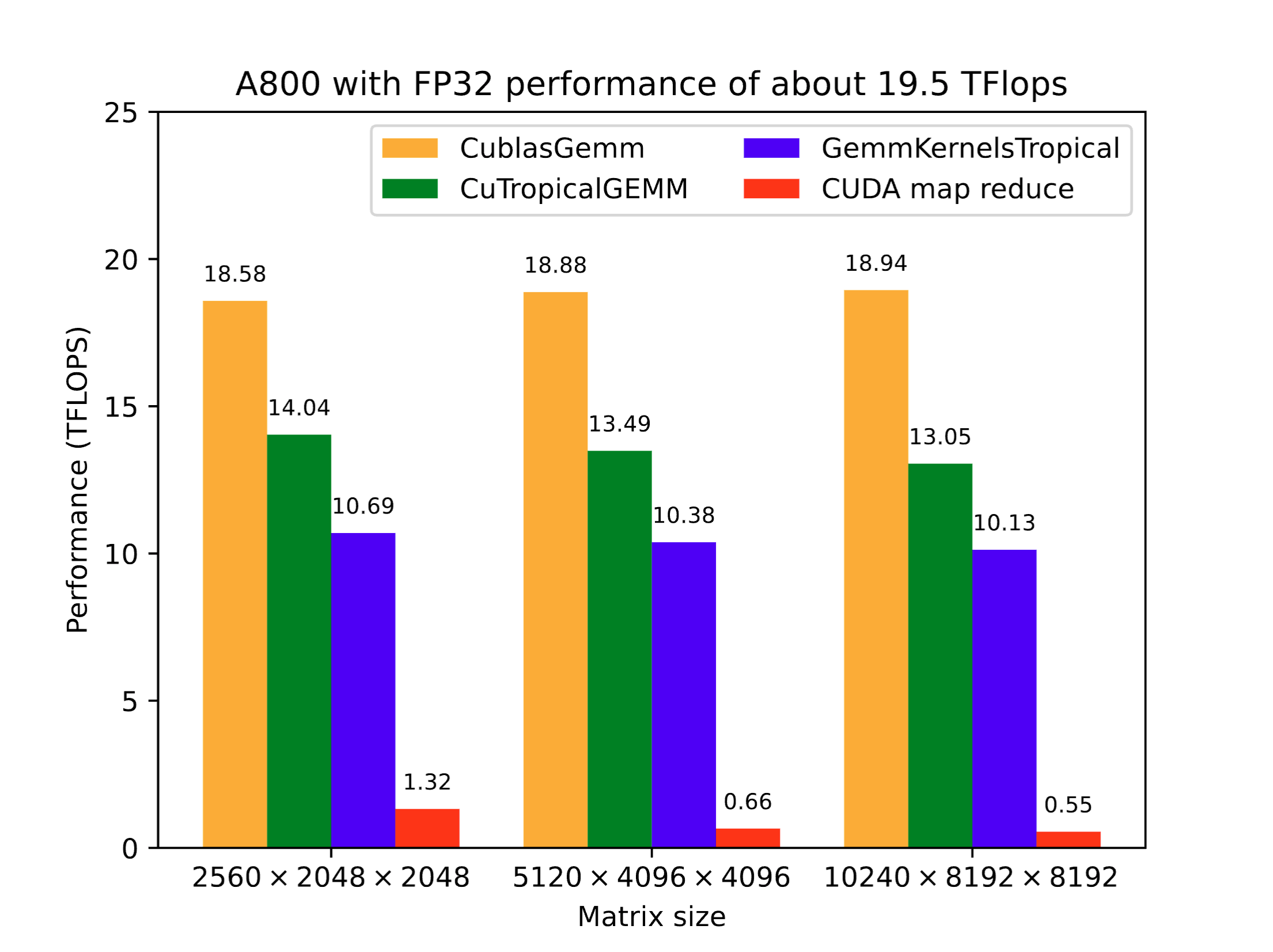 We compared the performance of
 CuTropicalGEMM.jl, GemmKernels.jl and direct CUDA.jl map reduce on Tropical GEMM with single precision. The performance is defined as
T2×M×K×N, where M, N, K are the size of the matrix so that 2MNK is the number of total operations in matrix multiplication, and T is the time cost. The performance of Cublas on normal GEMM is used as a reference of the maximum computing power. Clearly, the result shows that the performance of our package is about 75% of the theortical maximum, which is quite high since the tropical algebra can not use the fused multiple add (FMA) opeartions.
CuTropicalGEMM.jl can be easily used, just like the TropicalNumbers.jl. We fully used the multiple dispatch in Julia and overloaded the function LinearAlgebra.mul! for the types CuVecOrMat{Tropical}, which will be called when you use ∗ between these tropical vectors or matrices.
Here is an example:
julia> using CUDA, LinearAlgebra, TropicalNumbers, CuTropicalGEMM

julia> A = CuArray(Tropical.(rand(2,2)))
2×2 CuArray{Tropical{Float64}, 2, CUDA.Mem.DeviceBuffer}:
 0.5682481722270427ₜ  0.7835411877064771ₜ
 0.4228348375216514ₜ  0.9492658562534506ₜ

julia> B = CuArray(Tropical.(rand(2,2)))
2×2 CuArray{Tropical{Float64}, 2, CUDA.Mem.DeviceBuffer}:
 0.37361925746020586ₜ   0.6628092509923389ₜ
  0.3415957179381368ₜ  0.28749655890269377ₜ

julia> A * B
2×2 CuArray{Tropical{Float64}, 2, CUDA.Mem.DeviceBuffer}:
 1.1251369056446139ₜ  1.2310574232193816ₜ
 1.2908615741915874ₜ  1.2367624151561443ₜ
Or if you want to use a pre-allocate matrix C or calculate C+A×B, you can use:
julia> C = CuArray(Tropical.(zeros(2, 2)));

julia> mul!(C, A, B)
2×2 CuArray{Tropical{Float64}, 2, CUDA.Mem.DeviceBuffer}:
 1.1251369056446139ₜ  1.2310574232193816ₜ
 1.2908615741915874ₜ  1.2367624151561443ₜ
To benchmark the performance, you can use the @benchmark and CUDA.@sync marco.
julia> using CUDA, CuTropicalGEMM, TropicalNumbers

julia> A = TropicalF32.(CUDA.rand(4096, 4096));

julia> B = TropicalF32.(CUDA.rand(4096, 4096));

julia> @benchmark CUDA.@sync $(A) * $(B)
BenchmarkTools.Trial: 53 samples with 5 evaluations.
 Range (min … max):   6.691 μs …    1.574 s  ┊ GC (min … max): 0.00% … 0.00%
 Time  (median):      7.117 μs               ┊ GC (median):    0.00%
 Time  (mean ± σ):   29.701 ms ± 216.171 ms  ┊ GC (mean ± σ):  0.00% ± 0.00%

  █▅
  ██▅▃▃▄▃▁▁▁▁▁▁▁▁▁▁▁▁▁▁▁▁▁▁▁▁▁▁▁▁▁▁▁▁▁▁▁▁▁▁▁▁▁▁▁▁▁▁▁▁▁▁▁▁▁▁▁▁▃ ▁
  6.69 μs         Histogram: frequency by time         30.7 μs <

 Memory estimate: 256 bytes, allocs estimate: 7.
and what is important here is the mean time (currently there are some issues about the detection of time cost and we are still working on that).
You can also use that in more complicated cases, when developing you own package, by using CuTropicalGEMM, the mul! opeartions between Tropical matrices will be overloaded. Here is an example to directly use this package to speed up the maximum independent set (MIS) problem.
julia> using GenericTensorNetworks, GenericTensorNetworks.Graphs, CUDA, Random

julia> g = Graphs.random_regular_graph(200, 3)
{200, 300} undirected simple Int64 graph

julia> item(x::AbstractArray) = Array(x)[];

julia> optimizer = TreeSA(ntrials=1);

julia> gp = IndependentSet(g; optimizer=optimizer);

julia> contraction_complexity(gp)
Time complexity: 2^30.519117443024154
Space complexity: 2^24.0
Read-write complexity: 2^27.24293120300714

julia> @time CUDA.@sync solve(gp, SizeMax(); usecuda=true, T=Float32)
 31.104404 seconds (48.07 M allocations: 3.239 GiB, 2.31% gc time, 88.25% compilation time: <1% of which was recompilation)
0-dimensional CuArray{Tropical{Float32}, 0, CUDA.Mem.DeviceBuffer}:
89.0ₜ

julia> using CuTropicalGEMM

julia> @time CUDA.@sync solve(gp, SizeMax(); usecuda=true, T=Float32)
  0.361831 seconds (440.99 k allocations: 28.131 MiB, 85.79% compilation time: 100% of which was recompilation)
0-dimensional CuArray{Tropical{Float32}, 0, CUDA.Mem.DeviceBuffer}:
89.0ₜ
Here we will breifly introduce the techniques we used to speed up our code, which are commonly used in GPU implementation of GEMM. We learned a lot from the repo CUDA_gemm by Cjkkk. Here we will briefly introduce these techinques, and for more detailed introduction, I recommand this blog in Chinese.
As we all know, Nvidia GPU is fast because it have a large amount of cuda cores. For example, the Nvidia A800 GPU have 6912 cuda cores, which is much more larger than the number of CPU cores, which is normally less than 100. The peak flops of A800 is about 19.5T, which is also much higher than that of CPU, for example 0.5T for an Intel i7-10700K.
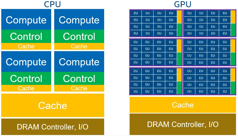
However, each cuda core is much weaker than that of CPU, so that the developer will have to properly allocate the tasks to these cores so that can fully use them. In a CUDA kernel, each cuda core is used by a thread and these threads are grouped as blocks.
Another imortant aspect is the memory of GPU, there are three type of programable memories on GPU:
Global memory, shared by all blocks, large but slow.
Shared memory, shared by threads in the same block, small but fast, just like a programable L1 cache.
Registers, used by only one thread.
Driectly loading data from global memory will take a long time, the bandwidth is only about 1000GB/s and the latency is about 600 cycles on A800 GPU. For shared memory, its bandwidth is about 20000GB/s while the latency is only about 23 cycles, so that another main target in GPU programing is to properly use the memory, avoid directly loading from the global memory and pre-load the needed data into the shared memory.
GEMM is a very memory-intensive operation, for example, when calculating the GEMM between a M×K matrix and a K×N matrix, if we use the naive way, i.e. evaluating the element in the result matrix one by one, for each element we will have to load 2K data, and there are M×N elements in total. Then we will have to load 2×M×K×N elements from the slow global memeory directly to registers in the whole process, and this generally far exceeds the data bandwidth of the GPU, resulting in serious performance issues.
To avoid the heavy data loading, we used the 'tiling' technique, which means we split the target matrix blocks into 'tiles' with size of BM×BN, and each GPU block will be used to calculate one of the matrix blocks, as shown in the fig below:
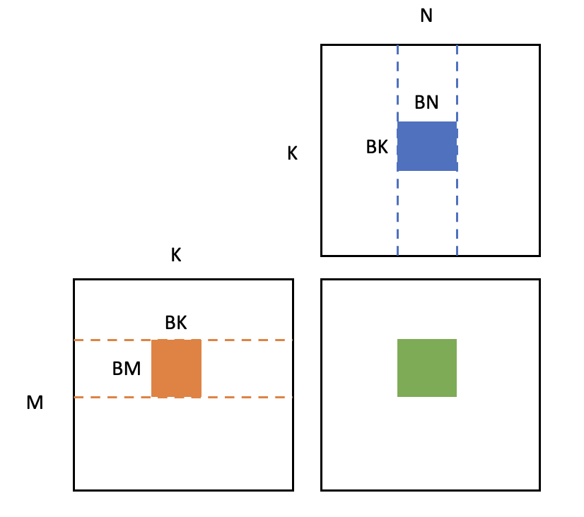
When calculating each block, we only need to load matrices with size BM×BK and BK×BN for K/BK times from global memory to shared memory. In that case, the total data loading will be reduce to
M×N×K×(BM1+BN1) which is much smaller than the naive way.
Then in each block, we further divide the matrix and use the registers to store the data, as shown by
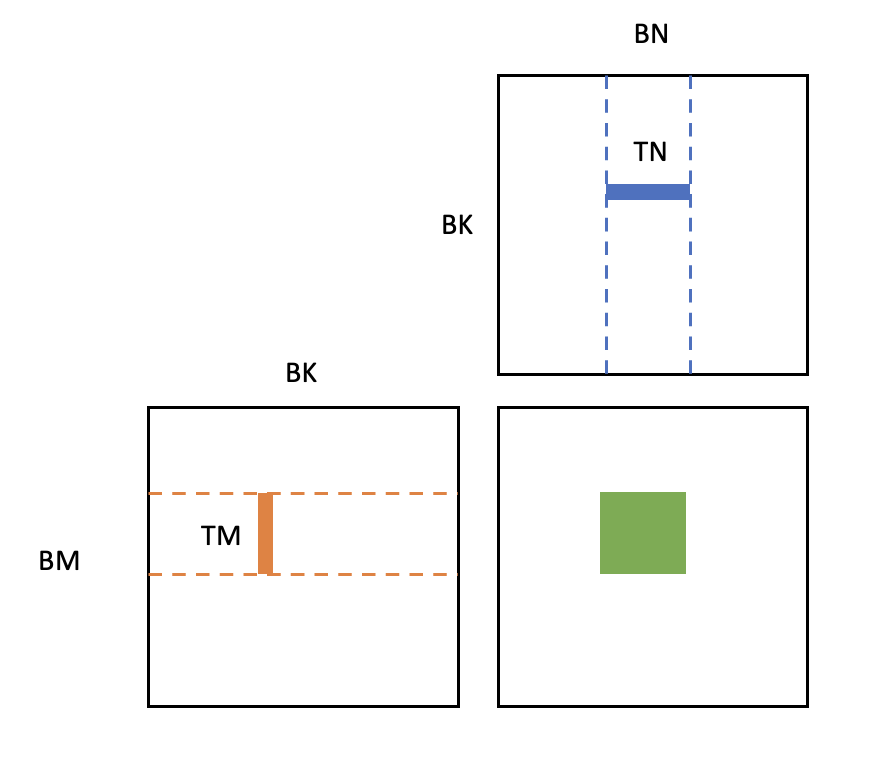
The target matrix will be further divided as small matrices with size TM×TN, and each thread will be used to calculate one of the matrix. During this process, the outer product way is used and data will be loaded from shared memory to registers, with the amount of (TM+TN)×BK in total. In our package, we set the parameters as
BM=64, BK=32, BN=64, TM=TN=4. As we mentioned above, the Tropical type is bitstype, and the data storaged in memeories are simply the floating point numbers, which can be directly used by CUDA kernels. Of course here we used the tropical algebra instead of the normal ones. Although the tropical algebra can not use the fused multiple add core (FMA), we found that the operation add/mul and max/min can be done on FMA and ALU parallelly, which means that we can use the FMA to do the add/mul and ALU to do the max/min at the same time. Then after all the calculation is done, the target in the registers will be stored back to global memory directly.
For the boundary elements, a padding strategy is used, we simply set the element which are not acctually in the matrix as the zero element of the corresponding algebra, so that they will not effect the result of the calculation.
Further benchmarking is still in development, and will be uoloaded to this repo CuTropicalGEMM_benchmark.
As mentioned above, this program is support by Open Source Promotion Plan 2023, JuliaCN.
Open Source Promotion Plan is a summer program organized by the Institute of Software Chinese Academy of Sciences and long-term supported by the Open Source Software Supply Chain Promotion Plan. It aims to encourage college students to actively participate in the maintenance and development of open source software, promote the vigorous development of open source software communities, and build the open source software supply chain together.
I will recommend anyone who is interested in developing open source software to join this plan. During the plan, the open source communities will release projects and each participant can choose three projects to apply. Once the application is approved, the participants can follow the mentor to complete the program in about three months.

I think it is a great chance to learn and to build connection with the community.
The plan starts in each summer, and the application commonly opens in June. If interested, just go and join OSPP 2024!
I am very grateful for the guidance and assistance provided by Prof. Jinguo Liu during the project implementation process. I would like to thank Tim Besard for his invaluable guidance and support during the development of the package, his expertise in GPU utilization have been immensely helpful. I also want to thank Tyler Thomas for his assistance in understanding the usage of BinaryBuilder.jl.